iCADdocs_online
Peak flood Estimation
Estimation of peak flood is solved using the SCSModel product. This module adopts conventional practice used to determine maximum probable floods using the SCS method of complex hydrograph. As main input variables, it uses:
-
Basic catchment properties (area and profile of the longest stream path)
-
Design Rainfall
-
Estimation method for Time of concentration
Table of Contents
- Conventions
- Typical workflow
- Technical Notes:
Conventions
- Profile data for longest stream path must be provided in ascending order (increasing distance for increasing elevation, or decreasing distance for decreasing order).
Typical workflow
A typical workflow for the use of the SCSModel module to estimate peak design flood is shown in the chart.
Prepare Object
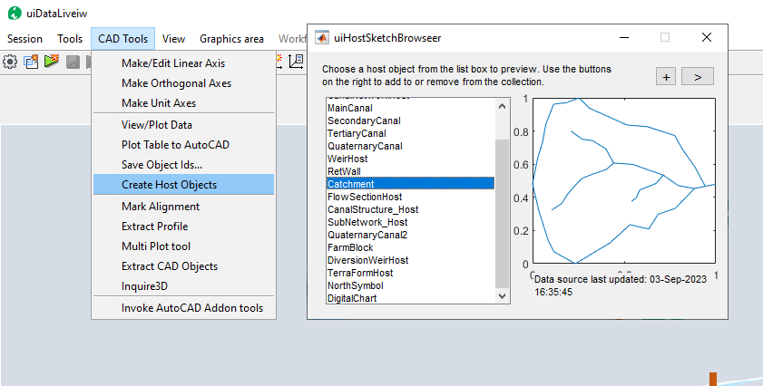
1. Start with a host object in AutoCAD, that represents the catchment object drawn using a polyline drawing tool. Tag the object to represent the catchment or basin label.
:bulb: Tip: Catchment host objects can be quickly generated from the There is no need to reference catchment object sketch.
- Provide stream profile data to the object. The data can be from a spreadsheet application, or CSV file. Copy the data, and use
Tools > Paste Clipboard to Object. - Follow the steps outlined in Data Processing and Presentation section to put the profile data to the catchment object.
Note: The profile data is an approximation of the profile data in a few segments as commonly practiced. It should not too long as in the direct extracted data from DTM sources.
Define Session and Start
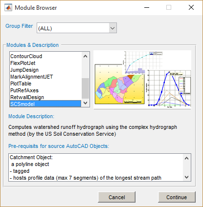
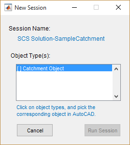
3. Define the session for the module from iCAD Session > Create and Run New Session. Select the SCSModel module, input the desired name for the session, accept and continue. The Catchment Object type is displayed in the Workspace Manager list box.
In the New Session dialog, click on the Catchment Object list item. AutoCAD will be in selection mode. Pick the catchment object prepared earlier. Back in the New Session dialog, hit Run Session.. This will start the module.
 {br}
{br}
Note: The Catchment Object will be marked [x] when associating the AutoCAD object is successful. The Run Session button is activated once the association is complete.
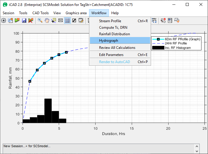
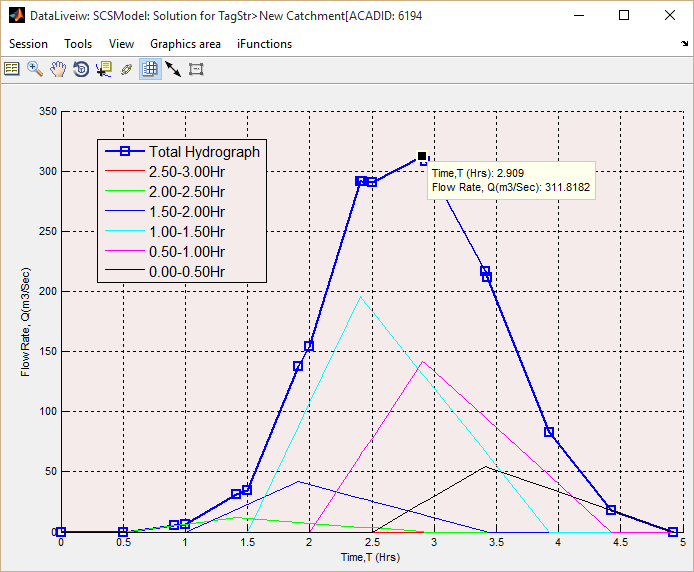
The module will start by displaying the rainfall distribution curve for the catchment.
 {br}
{br}
Explor the hydrograph solution from Workflow > Hydrograph menu command.

Edit Variables
The results displayed are determined from the default settings. Edit the parameters from Workflow > Edit Parameters or CTRL+E to suit the specific catchment condition under investigation, as detailed below.
Edit default variables using iFunctions > Edit Variables as shown below. Then click Apply button to solve.
| Group | Variable Name | Description and Remarks |
|---|---|---|
|
Design Peak Rainfall (mm) | The 24Hrs recurrent (e.g., 50Yrs, 100Yrs) design rainfall |
| Catchment Area (Km^2) | The area of the basin in square kilometers | |
| Curve Number | SCS curve number for the catchment♣ | |
|
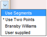 Tc computation method Tc computation method |
Choose desired method for computing TC values:
|
| Set TC value (Hrs) | A user set value for time of concentration. | |
| Incremental Duration (Hrs) | Duration interval for the computation of the triangular hydrographs for each incremental duration rainfall in the computed rainfall profile. Choose from:
|
|
| Temporal profile method | Method for determining the temporal variation of the 24Hr rainfall. Choose from:
|
|
| Area Reduction method | Method to be used for changing point rainfall to area rainfall. Choose from:
|
Note: The curve number corresponding to proper antecedent moisture condition must be used.
The first two methods use the Kiprich’s formula. (See note below for details)
Explore the solution
Explore the solution by varying calculation methods and parameters to find a representative and fit solution to the design task. Use Workflow > Compute TC, DRN menu command to compute Time of concentration using all four available methods.
A tabular presentation of results is also available in the Table View interface as shown below.
Technical Notes:
Time of concentration is estimated using one of two methods, namely the Kiprich’s formula, and Bransbey Williams Equations respectively:
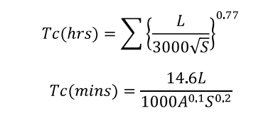
Where L is horizontal distance (m), S is average slope of segment (m/m) and A is the catchment area in square kilometers.
The peak flood is derived from the 24Hr design rainfall magnitude.
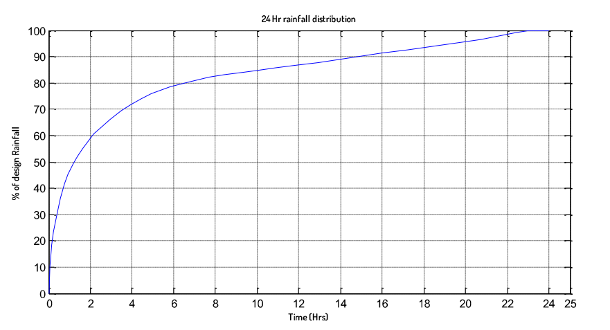
Temporal distribution of the design rainfall is approximated using one of two available options. The first option uses this equation:
 {br}
{br}
Where P is the recurrent design rainfall (mm).
The second option uses the above chart to determine the distribution over 24Hrs period.
 {br}
{br}
Spatial variation of the point rainfall is estimated using the Area to Point ratio relationship. Two options are available.
1) Tabular data (built-in) relating corrections for depth of rainfall as a function of incremental duration and Catchment Area (Such as found in the IDD manual). Factors are applied to catchment areas >25sq.Km.
2) Using the following empirical relationship:
 {br}
{br}
Excess rainfall is estimated using the following common relationships in litrature:
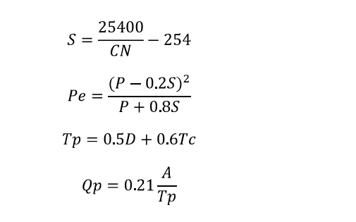 {br}
{br}
Where:
-
Tc is time of concentration (hrs),
-
D is incremental duration (hrs),
-
Tp is time to peak (hrs), and
-
Qp is excess rainfall(mm)