iCADdocs_online
Data processing, analysis and presentation
CAD offers a number of tools for data processing and visualization. The tools are selected to fill practical data visualization and presentation challenges in every day design tasks.
This page presents each tool available, and how to use it to tackle design challenges. Use table of contents outline below to navigate through this page.
Table of Contents
- Summary of functions
- Host Data to AutoCAD Objects
- Plot Data in to AutoCAD
- Plot Graphic elements to AutoCAD
- Plot Text Table to AutoCAD
- Local Coordinate system and Object Referencing for iCAD use
- Drawing Results to AutoCAD
- Create and Edit Alignment Markers
- Generating profile data for Alignment routes
- Data Visualization and Presentation
- Using CAD Objects Extractor
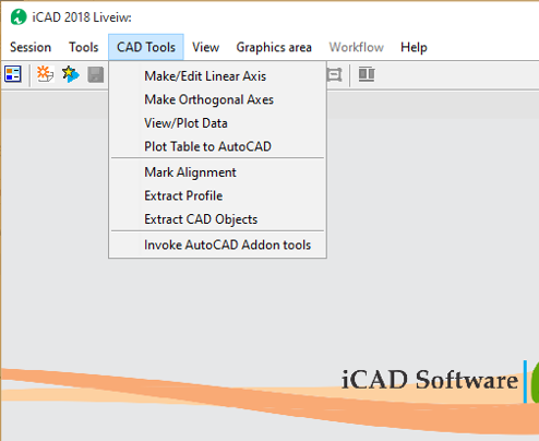
Summary of functions
Functions for preparing data and AutoCAD objects are available either as CAD Tools in iCAD, or embedded AutoCAD utilities also called AutoCAD Add-on utilities.
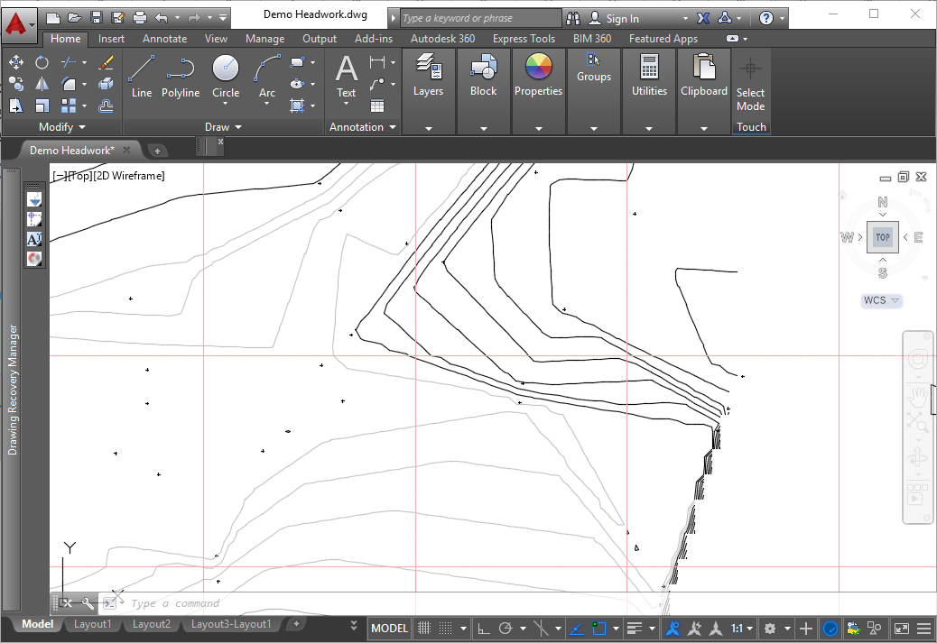
AutoCAD Add-on utilities shown on the left of the AutoCAD model space.
The utilities allow power users to exchange data from iCAD to AutoCAD and back to iCAD, while also allowing easy annotation and rendering of drawing details with in the AutoCAD environment.
The following are the key funcitons available for use in iCAD/AutoCAD environment.
-
Paste Data: Transfers data from an Excel workbook to an iCAD process. View Data displays hosted data on objects.
-
Alignment Profile: Creates a strip profile from a 2D layout (route) object and using cloud of spot data.
-
Marking and Referencing Functions: Allow to mark, label and reference AutoCAD objects to cater for modules in iCAD environment.
-
Plot/View Data (FlexPlotJET): A versatile plotting/viewing function. It can be used to render analysis and solution to AutoCAD environment. It has a capability to render table data, as well as graphic components from iCAD’s DataLiveiw interface. It can also be used to visualize, and process data before exporting to AutoCAD.
Note: FlexPlot handles a maximum of 10 data series at once, and can position/label a maximum of 100 tick marks (on an abscissa or ordinate measure.) The user is warned if more than 50 tick marks are encountered. During Object (coordinates) import to iCAD, the current version allows up to a maximum of 120 vertices with an accuracy of 10^-8.
-
Table Plot: Plot tabular data as a table in to to AutoCAD.
Note: Only numeric columns are plotted to AutoCAD.
A typical set of tasks that can be accomplished using tools and functionalities are presented below.
Host Data to AutoCAD Objects
One of the power features of iCAD is its ability to enhance the use of AutoCAD environment as a true design environment by allowing objects to host raw data or relevant processed data.
A common source of raw data is a tabular data from Excel, such as shown here. Another example is the spot data collection from surveying work detailing topographic variations of a development area. Hosting these data on AutoCAD objects makes them easily available and accessible during later analysis and generation of derived data such as contour maps and profile plot.
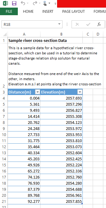
We will show how to host this data on an AutoCAD object for latter use.
Before proceeding, follow these steps to make sure to observe the following Important conventions: for a successful operation to prepare the data with in Excel, or Notepad (CSV format), or OpenOffice spreadsheet.
-
All columns must have headers.
-
Headers must have no spaces, and can only no symbol other than the open or closed bracket symbol.
-
Data table below headers can ONLY contain numbers. No text or string data is allowed.
-
Data can have any number of rows or columns.
-
The data must be copied along with the header information.
Then follow below typical workflow:
-
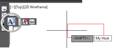
Prepare the Object in AutoCAD. Draw an arbitrary object using the AutoCAD polyline command. Use the Attach Tag addon tool to give it a recognizable name.
-
If your data is in a file, skip this step. To use windows clipboard, open the data in excel environment, select data and copy using
CTRL+Cshort cut. -
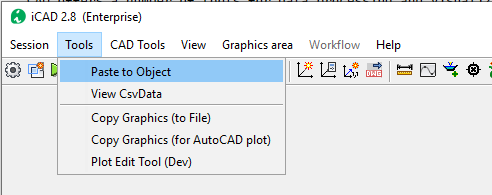
Start the menu command from ‘Tools > Paste to Object` from iCAD interface.
-
In the dialog, pick
FileorClipboarddepending on your data source locaiton.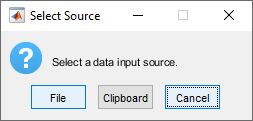
-
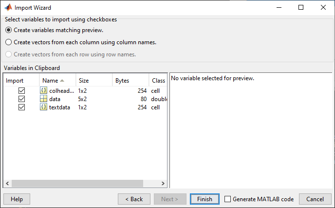
The import dialog starts, showing a preview of the data in the clipboard. Accept
NextandContinuebuttons.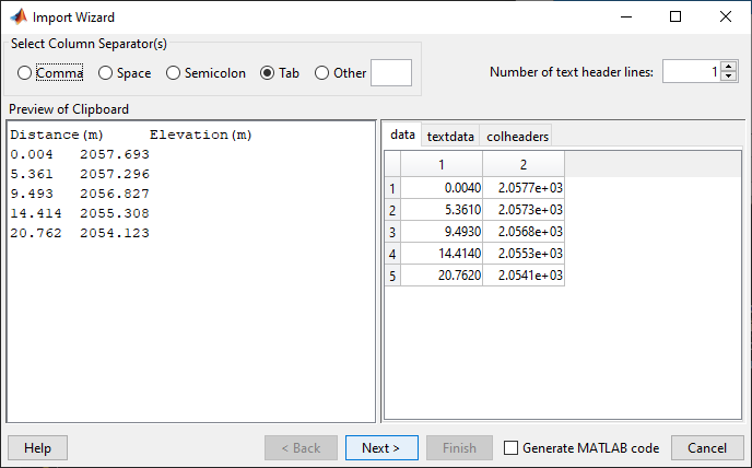
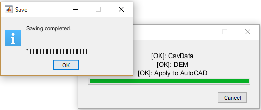
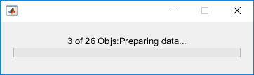
 {br}
{br}Note The status bar at the bottom of the main iCAD interface (above). If successful, it reports the paste operation is completed.
To view stored data, follow below steps.
-
Go to
Tools > View CSV Data.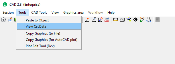
-
Go to AutoCAD and pick the host object. The status update bar reports if a data is found or not.
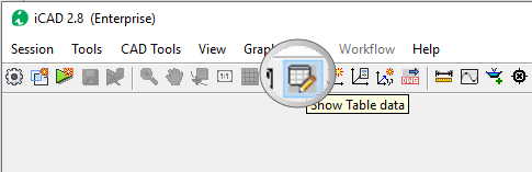
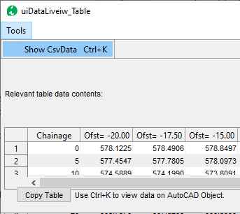
The data is presented in the uiDataPreview table. Toggle its visibility from the Show Table Data toolbar button.{br}
Alternatively, you can use the menu command in Data Table View interfac, and repeat step 2 above. The data content of the table is updated accordingly if found.
:notebook: Technical Note: These data are saved in CSV format in the accompanying AutoCAD file to the project (*.xsd). They can not be edited. However, they can be replaced with modified data any time.
Plot Data in to AutoCAD
One of the most needed functionalities is the ability to render plots of data, analysis results and even graphic objects in to AutoCAD environment with ease. In iCAD, this is achieved using the FlexPlotJET modile – a powerful and versatile plotting utility used by all other modular solutions. Data sources for this operation can be either of:
-
Windows clipboard data. These can be from:
-
copied from Excel, or Notepad (CSV format), or openOffice spreadsheet.
-
tabular presentation of other iCAD solutions, or
-
graphic data from DataLiveiw interface copied using Tools > Copy Graphics (for AutoCAD Plot) menu.
-
2) Hosted data in AutoCAD object such as pasted raw data as explained in previous function or results of analysis such as from a stream rating curve analysis.
A typical workflow to plot data using this function is as follows:
-
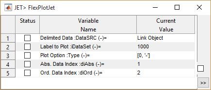
Invoke the solution from iCAD Explorer Tools > Plot Data to AutoCAD menu. This will bring the input dialog.
-
Specify the data source in the first row. Click on the Link to object… cell to pick an AutoCAD object hosting the data to be plotted. Shift click on Link to Object… cell to type cb or clipboard and use the data on windows clipboard.
:bulb:Note: For cliboard source, make sure the source data is prepared in an Excel workbook, and the first row contains acceptable data header strings.
-
Specify which data columns are to be plotted on the abscisa and ordinate axis, and select the plot type.
-
Accept all inputs and proceed.
-
A dialog box will appear asking for the plot area. Select the desired destination from the options.
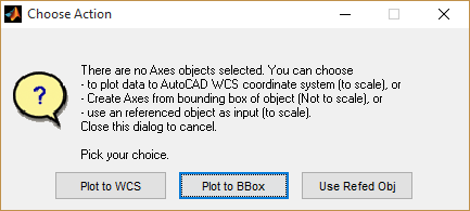
Note: Plot to WCS plots the data to AutoCAD World Coordinate System (WCS). Plot to BBox allows users to select an object whose top-right and bottom-left coordinates are essentially different and are used to define the plot area. Use Refd Object option allows to pick an existing object
-
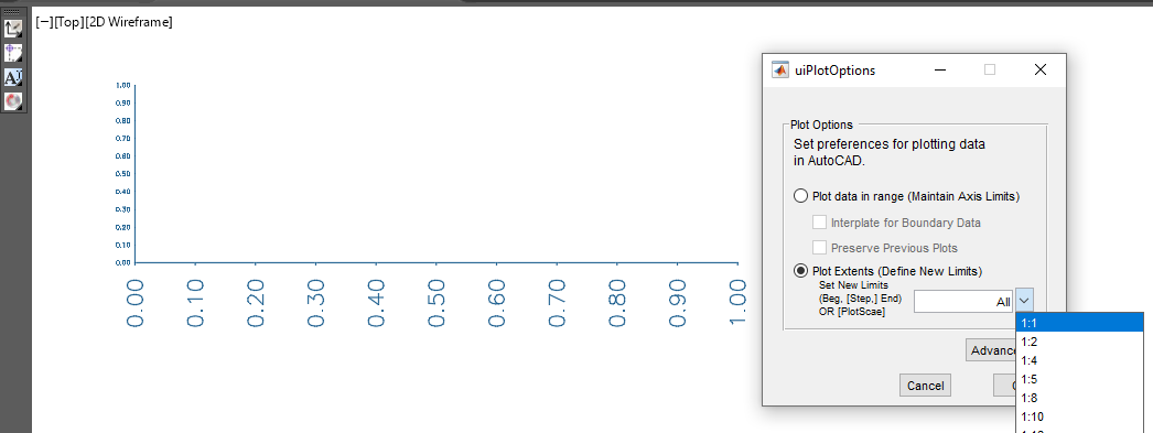
Specify plot options on the next dialog.
-
Accept the All option for a fit-to-area plot of your data.
-
Specify a plotting scale >0 to define a common plotting scale for both horizontal and vertical axes.
-
Input a negative value to specify the plot scale latter in the plot process.
The data plot is generated in AutoCAD environment as desired.
:bulb: Note: FlexPlotJET handles a maximum of 10 data series at once, and can position/label a maximum of 100 tick marks (on an abscissa or ordinate measure.) All data in excess of 10th series are ignored. The user is warned if more than 50 tick marks are encountered. During Object (coordinates) import to iCAD, the current version allows up to a maximum of 120 vertices with an accuracy of 10^-8.
Edit, annotate and enhance plot using iCAD and inCAD utilities.
- Edit axis tick marks, labels, scaling and more using
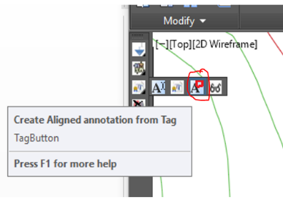
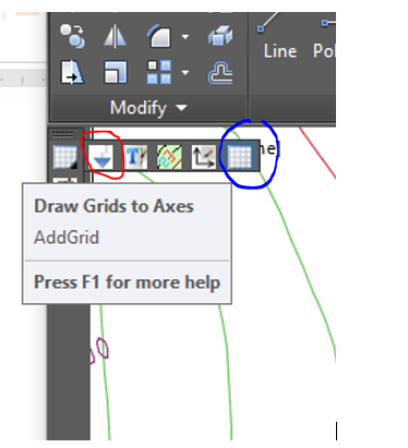
CAD Tools > Edit/Make Linear Axismenu command. - Add grid lines using the Mark Curves and Draw Grids to Axes addon tools from with in AutoCAD (shown above)
-
Plot Graphic elements to AutoCAD
Most modules create graphical information on the main interface area of iCAD. These data represent solutions to specific to the modules. The user can export these data in two ways:
Save to a File
To save the graphic areas as is for documentation purposes follow below steps.
-
Start
Tools > Copy Graphics (to file)menu command.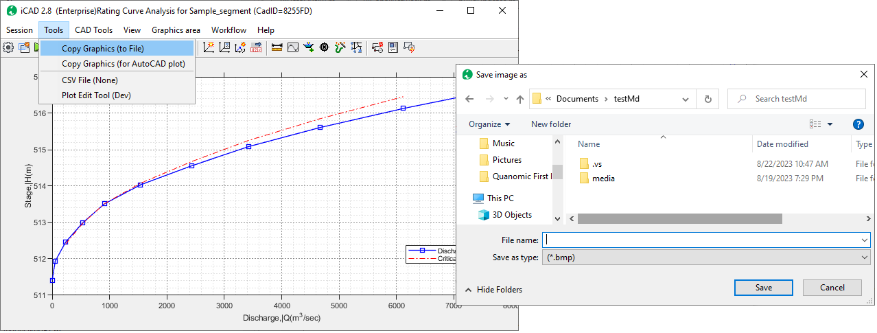
-
In the save as dialog specify the locaiton and file name for the image, and hit
Savebutton.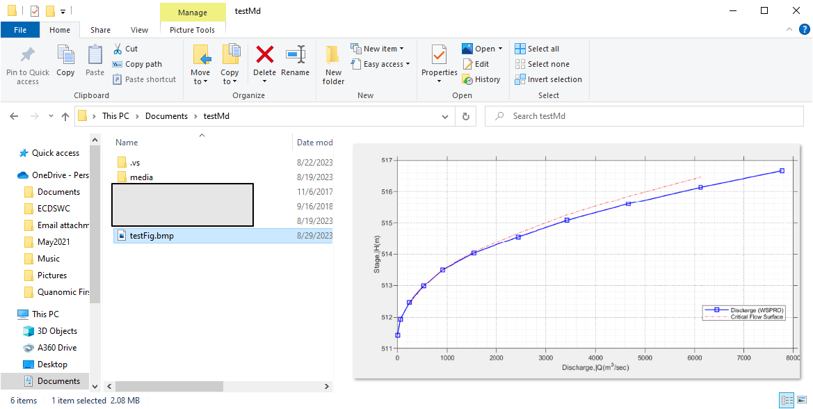
The file can now be used as any other image file.
Generating to AutoCAD
A drawing of all the graphic elements can be generated to AutoCAD with or with out scaling as needed. To generate drawings, follow these steps.
Note: iCAD generates drawings to the currently linked AutoCAD file. Make sure there are no multiple files opened, or at least you do not point to another file. This may cause your AutoCAD application to Crash.
-
Start the
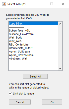
Workflow > Render to AutoCAD...menu command orCtrl+’P’ short cut. This will list all objects in the graphic area grouped by tags.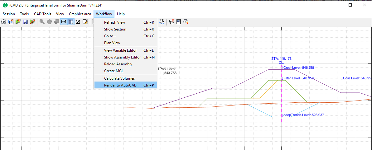
-
In the Select Groups dialog, select the Copy BBox group. This will create the reference axis and object required for plotting. On the next dialog, choose Plot to BBox, and hit
Continue.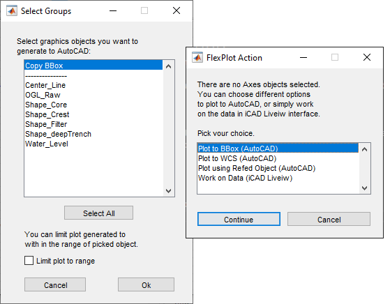
-
AutoCAD will be in select mode, requiring to select a bounding box area to position the ploted autocad objects. If not prepared, click on a blank area. Dont mind the Invalid Pick dialog. Prepare the rectangle. Now back in the dialog, hit the
Retrybutton.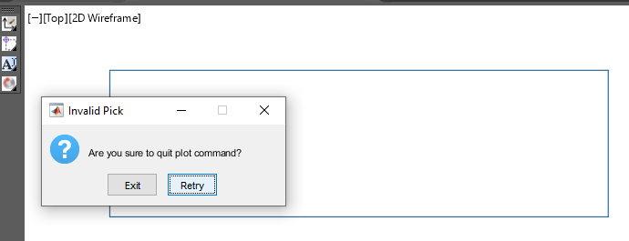
-
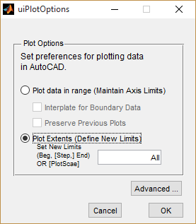
The axis creation process beings with default settings. Specify how to plot the data and the scaling in the uiPlotOptions dialog. This will complete the axis creataion.
-
Back in iCAD, restart the process from
Ctrl+’P’ or the menu command as in step 1 above. This time, select all tag groups or the ones you desire. UseShift+Clickto selectively pick groups.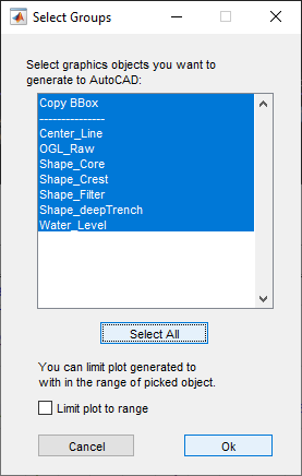
-
AutoCAD will be in select mode. Click on the diagonal object created in earlier step. This will serve as a refernece object to position and scale the new plots.
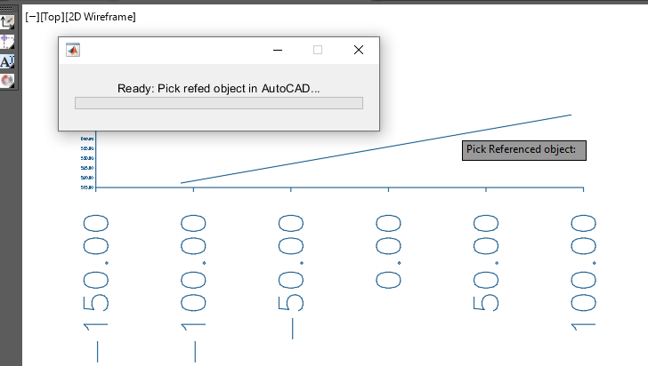
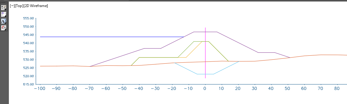
All the objects are now generated in the AutoCAD environment. The image below is after some axis editing as explained further below here.
Plot Text Table to AutoCAD
Similarly, you can plot tabular data as a table to AutoCAD. The data sources for this task can be similar to those for the plot data function above. In addition, DataTable contents from any of iCAD’s modular solutions can be used as a source.
The workflow to using this function is:
-
Invoke the function from CAD Tools > Plot Table to AutoCAD. A dialog box appears asking for a Dump Object, the area to place the table in AutoCAD. This is similar to the bounding box concept used in making axes. Click on the Link to Object cell to select an object that indicates an area to render the table data in AutoCAD. (shown in red in this example.)
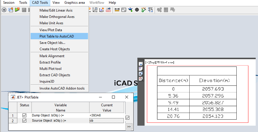
-
Shift+Left-Clickon the Link to object cell of the Source Object variable, and type in cb to use clipboard data. If the data is hosted in an object, simply click and link as step one above. -
Hit the
>>button.
The table is generated in AutoCAD.
:bulb: Tip: AutoCAD uses the current text, color and other settings to generate the table data.
:warning: Note: only numeric columns are plotted to AutoCAD using this tool.
Local Coordinate system and Object Referencing for iCAD use
AutoCAD model space uses its own coordinate system to reference and position objects. There are two types of coordinate systems. The WCS or World Coordinate system is the fundamental coordinate system referencing all objects in the AutoCAD model space globally. The UCS or User Coordinate System on the other hand is created by the user to create a local reference axis. This coordinate system allows to (re)locate an origin of a user coordinate systems anywhere in the model space.
iCAD adopts a similar coordinate system as the local coordinate system to reference and position objects, such as design charts or drawing components. The unique advantages of the iCAD created coordinate systems are:
-
Multiple reference axes (or coordinate systems) can be placed on a single drawing file, and all can be used simultaneously, and independently of each other. (in contrast to the AutoCAD UCS tool)
-
iCAD coordinate systems are planar (i.e. X,Y system)
-
iCAD coordinate systems can have different scaling in x and y direction.
Referencing AutoCAD objects to a local axis allows syncing coordinates of existing objects to enhance use of spatial information and facilitating positioning of subsequent new plots. Three basic tasks are outlined below: thus (a) creating local axis, (b) referencing objects to axes system and (c) creating additional axis.
Create and Edit floating Axes
Floating axes are not linked to any reference. They are placed randomly, and represent arbitrary range of data.Floating axes creation and editing tools in iCAD can be invoked from the menu commands shown below.
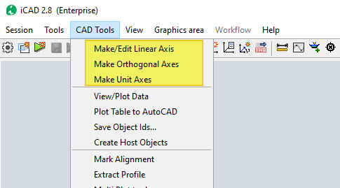
They can also be invoked directly from the toolbar menu.
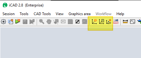
The toolbar items are, from left to right, for New Axis creation, Editing an existing Axis, and creating a unit axis.
One can create new axes, or edit existing axes for their details as shown below.
Create a new axes
-
Start the menu command from
Cad Tools > Make Orthogonal Axes. -
In AutoCAD, pick the object defining the bounding box for the axes area.
-
The variable editor dialog appears. Set axis limits for Abscisa and Ordinate as desired.
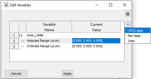
WCS data: Uses the AutoCAD World Coordinate System the object is located to create an axis. This will enlarge the BBox a little to set starting and ending positions.
Ref Data: Use this if the object selected for the bounding box is referenced to a an existing axes pair. All objects (except Host objects) created by iCAD and CanalNETWORK are by default referenced to an accompanying axes.
User: This option lets users define their own start and end for both vertical and horizontal axis.
Note: The value sets are START, STEP, END.
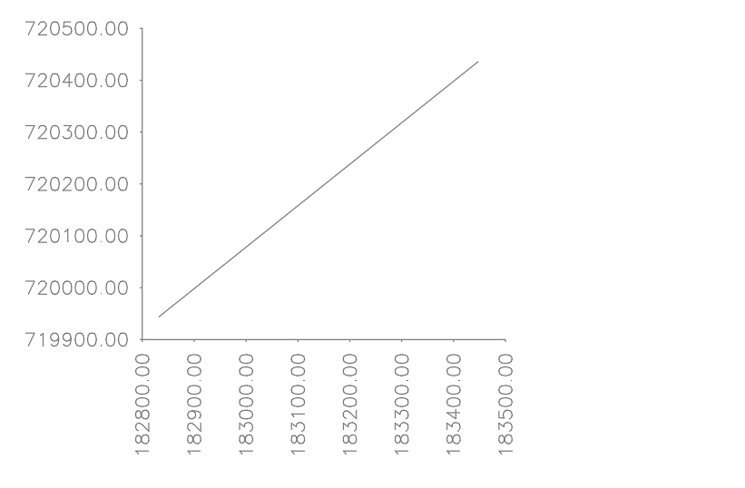
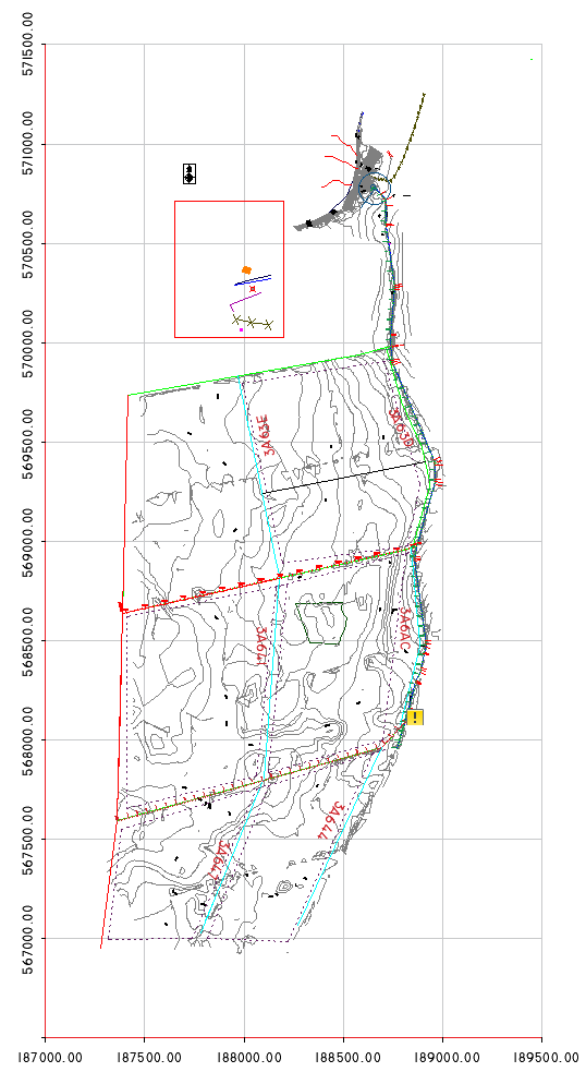
An axis from a diagonal line used as the bounding box, and using AutoCAD WCS option.
Editing Axis
The appearance and orientation of axis labels can be changed as follows.
-
Start the menu
CAD Tools > Make/Edit Linear Axis... -
In the dialog, ckick on the first row second column cell, and pick the axis to edit in AutoCAD.
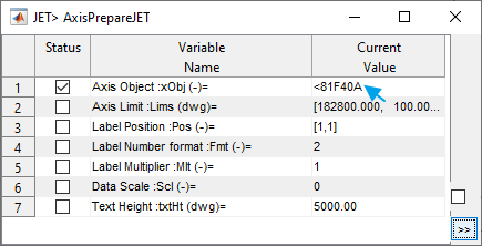
-
The dialog box populates the values of the current setting in the box. Edit as desired.
-
Axis Limits: START, STEP, END (step is not always applied and depends on the size of the axis)
-
Label Position:
-
[1, 0] Left: put labels on left side, (refernce counterclockwise to the box),
-
[1, 1] Left Rotated: as above, but rotated to 90deg.
-
[-1, 0] Right: put labels on right side, (refernce conterclockwise to the box)
-
[]-1, 1] Right Rotated: same as above, but rotated to 90deg
-
-
Label number format: specify how many decimals to use for axis labels.
NB: It is not recommended to change below data, especially for axis contaning referened plots.
-
Data Scale: Input if specific scaling is required for the axis. If 0 (default), then the axis limits (NOT the data) will fill the bounding box. If a >0 is input, both x and y axis will be scaled to that value. a value of 1 can be used to generate 1:1 scale drawings from the graphic in the main iCAD interface.
-
Text Height: Leave the maximum number to allow automatic sizing of texts. But can be set to a desired value as well.
-
Upon completion, the axis will be redrawn in AutoCAD with the new changes.
Creating Unit axes
A unit axes is a pair of orthogonal axes, whose data limits in both the x and y direction are [0, 1]. These may be required for varying reasons.
To create a unit axes:
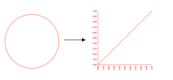
- Draw a bounding box object in AutoCAD. If similar scaling is required in both x, and y direction, use a circle or a square.
- Start
CAD Tools > Make Unit Axes. The Flex Plot Action dialog appears. -
Select Plot to BBox (AutoCAD) option, and hit
Continue.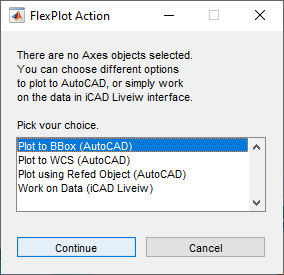
- AutoCAD is in select mode. Pick the circle object.
This will generate the desired axis, deletes the circle object, and creates a diagonal refernced object.
- In the Edit Variables dialog, set the Abcsisa and Ordinate range variables to User, and leave the default [0, 1] on both.
Creating Referenced Axis
Referenced axes, in contrast to floating axes, are linked to the AutoCAD World Coordinate System (WCS). These create axes and data limits pertinent to the location where the bounding box is located with respect to the WCS.
To create a local axis system anywhere in the drawing space:
-
Draw a rectangle, circle or diagonal polyline whose bottom left and top-right coordinates are used to define the limits (commonly referred to as the bounding box or BBox in iCAD documentation) of the axes to be created.
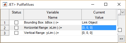
- Invoke CAD Tools > Create Orthogonal Axes. The JET input dialog appears. Assign the variables as follows:
- Click on Link Object value cell, and go to AutoCAD to pick the BBox object created above.
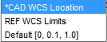
- Choose CAD WCS Location.
- (optional) Do the same for the Vertical Range: yLim variable.
- Hit the
>>button to continue. The iCAD local axes will be generated around the BBox object using the AutoCAD location values.:bulb: Note: The actual axes may be slightly larger than the original bounding box object. This is because the axes MUST start at a whole number convenient for presentation, and not where the box is arbitrarily located.
Referencing objects to an Axis system
There are two methods to reference polyline objects to an iCAD local axis - from a axes, and from previously referneced objects.
To reference any object to an axes pair:
-
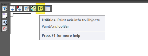
Select Utilities-Paint axis info to Objects utility as shown.
AutoCAD will prompt to pick the reference axes.
- Pick the horizontal and vertical axis consecutively.
-
AutoCAD will then ask for the object to reference. Select the polyline object (or multiple polyline objects one at a time) and right click to finish selection. AutoCAD will confirm succefully referenced at the status bar.
NOTICE
- ONLY polyline objects are accepted for referencing with iCAD local axes.
- The number of objects successfully referenced is displayed in the AutoCAD command prompt.
Once can also reference objects by using previously referenced objects. If already referenced objects exist, then this method is slighly faster:
- Start the command Utilities-Paint axis info to Objects from the Addon toolbar.
-
Instead of picking a Horizintal axis, as prompted by AutoCAD, hit the ↓ (down arrow) on the keyboard, and select
Copyoption. AutoCAD will prompt for the base referenced object. Pick the existing referenced object. - Click on the new object or objects, and right-click when done. All objects are now referenced to the base axis to which the base reference object is referenced.
 AutoCAD will confirm successfully referenced objects on the command line.
Drawing Results to AutoCAD
Any solution on the main interface can be sent to AutoCAD for scaled drawing and further processing. This is made possible in one of two ways.
1. Using Menu command
The first method is to use the menu command available for each session under the Workflow menu.
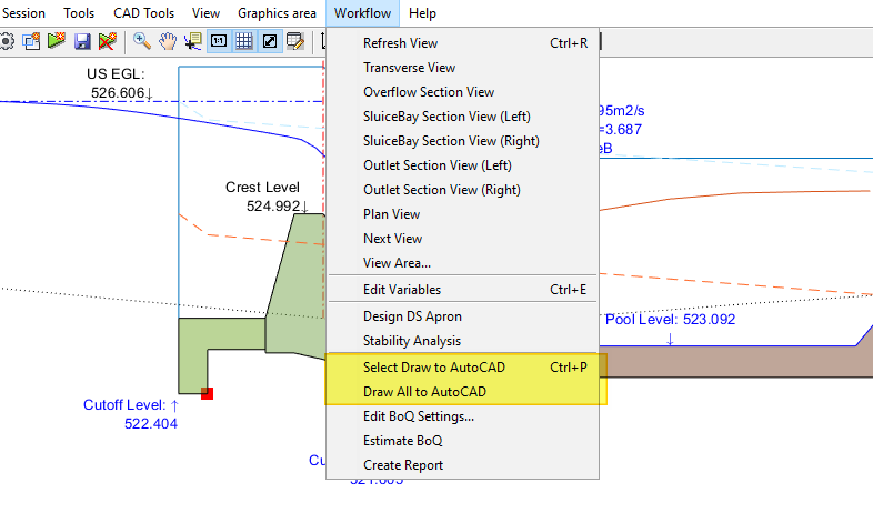
Choosing the Select Draw item allows to draw elements of the results selectively. It will invoke a dialog that allows to pick items for sending to AutoCAD.
Select any set of objects and hit Ok to continue. AutoCAD will be in select mode. Pick a refernced object in an already existing axis to continue.
:exclamation: Important Note: Do not select a plotted object, whose coordinates are trimmed (see method 2 below), or the plotted objects will shift.
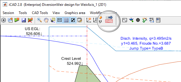
2. Using the Toolbar Command
One can draw to AutoCAD using the toolbar item command. This tool invariably generates all the displayed graphic elements to AutoCAD.
As opossed to above method which requires a referenced object, this tool also generates its own local axis system to plot the elements. On start, pick a bounding box object in AUtoCAD. The rest will be automatically completed.
:bulb: Note: VIsible elements, with in the boundary of the view port, are creatd in AutoCAD. Elements extending beyond the current axes limits (view area) will be trimmed for their X values before sending to AutoCAD>
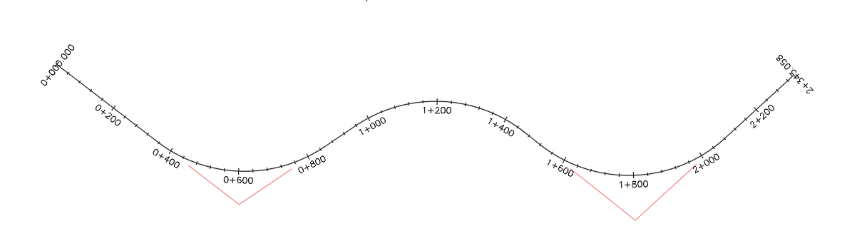
Create and Edit Alignment Markers
An alignment line is a polyline object drawing in AutoCAD that represents a layout instance of a canal route, or similar. Marking an alignment is the task of putting station markers along the alignment at specified intervals and text orientation.
To create markers along an alignment use below steps:
-
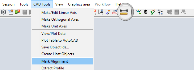
Start the menu
CAD Tools > Mark Alignmentmenu command, or the tool bar option. AutoCAD will be ready in select mode, promoting Pick Alignment object to Mark: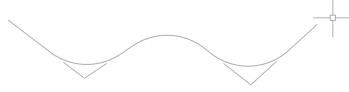
-
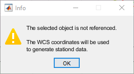
Pick the object for marking. If the object is not referenced, a dialog will apear to confirm the process. Accept and continue. If not, it will continue.
-
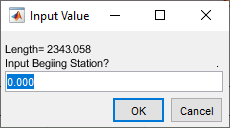
If the Alignment has longitudinal informaiton, it will continue to step 4. If not, a dialog will apear to confirm. Accept
Set New. Input the deisred starting station for the object.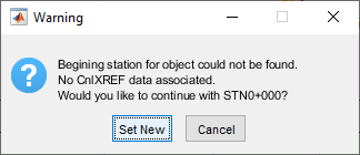
Markers are created using default settings.
Start the command again, and select the marked alignment to edit the specification for the markers.
-
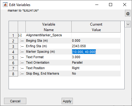
Upon selection of a marked object, the below dialog appears to change how the markers are displayed.
-
Begining Station: Starting marker value.
-
Ending Station: Ending marker value.
-
Marker spacing: Minor and Major Steps for marking the alignment. Major marker locations bear text information, while minor marker locaitons are drawn as simple ticks.
-
Text Format: [A.B notation] A represents the location of + sign on station markers, and B represents the number of decimal places to use when generating station tetxts. For example, for station value of 12345.3456:
-
3.0 will give 12+345
-
3.2 will give 12+345.34
-
0.3 will give 12345.345
-
-
Text Orientation: Parallel orientation rotates anotation texts parallel to the alignemnt object, while Perpendicular rotates them to appear normal to the alignment.
-
Text Position: Specified whethter text is to be put to the right or to the left of the alignment object.
-
Skip Beg/End markers. If editing markers on plan views, the end markers are automatically generated and need not change. Use this option to skip affecting them.
Partial stations can be marked by specifing statting and ending stations accordingly. For the above example, using 300, 900) will work out as below.
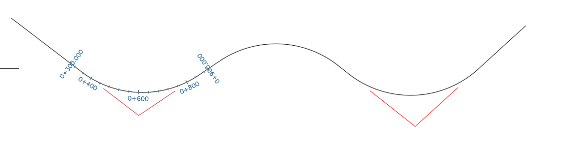
-
Generating profile data for Alignment routes
The solution CAD Tools > Extract Profile or CTRL+F invokes the modular function that creates a strip profile from a 2D layout (route) object and cloud of spot data. Such data are the starting points for many other iCAD modules including CanalStructures, JumpDesign and RetwallDesign among others.
Conventions
-
Station distance increases from beginning to ending vertex.
-
Offset is left (-ve) to right (+ve) face-upstream or facing opposite the direction of station increment.
-
Elaborate full process with relevant content (Succinct)
Extracting and displaying profile data
Alignment objects should be drawn using the polyline object tool on a contour plot and reference it. Prepare the alignment object in this manner and:
-
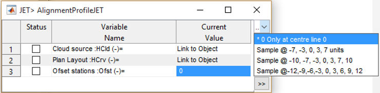
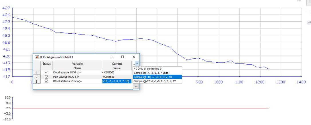
Invoke the CAD Tools > Extract Profile module. When the JET dialog appears, set the values of each variable as appropriate.
-
Link an object hosting cloud of spot data (the surveyors list of x,y,z pairs) to the Cloud source variable.
-
Link the referenced alignment route object to the Plan Layout object.
-
Select the desired offset settings from the dropdown list, or provide a different offset specification.
Tip: The notation [start: increment: end] can be used to specify offset locations. [-2:1:3] for instance is the same as [-2, -1, 0, 1, 2, 3].
Note: Offsets are specified from left to right, facing towards the beginning of the alignment object. For profile alignment along a river centerline, for example, the offset is specified from left bank to right bank, facing upstream.
Note: The module can generate strip profile for a maximum of 29 transverse data points.
Note: The cloud data source should be referenced to an iCAD generated local axes system.
Tip: Use 0 (or defualt *0 Only at center line to generate data along the center only.
Accept the input values, and hit
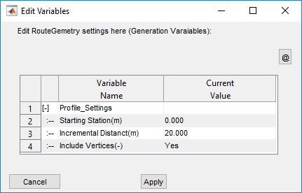
>>to continue. Provide further inputs in the Edit Variables dialog as follows: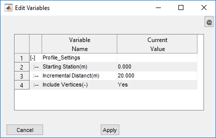
-
Starting Station (m): Input starting station for the alignment route. Default is 0.00
-
Incremental Distance (m): The desired spacing between successive profile data points. Default is 20m interval.
-
Include Vertex (-): Specify whether to include vertex points of the alignment in profile data. Settings Yes forces data to be read at vertex points. If No is used data points are extracted only at incremental locations.
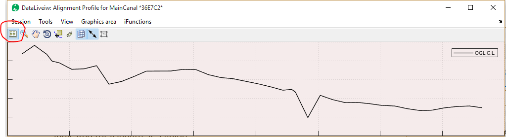
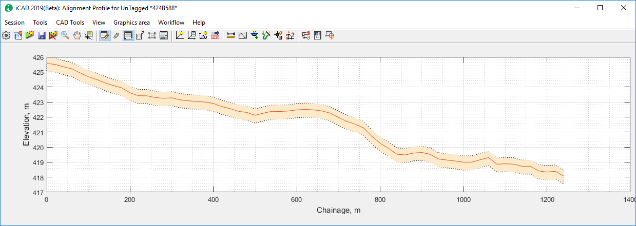
Click Apply to preview the profile data.
-
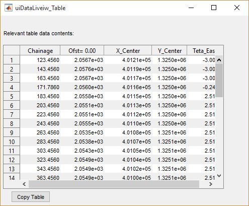
-
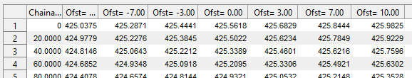
Click on the Data Table toolbar in Data Liveiw to get the numerical data for further use.
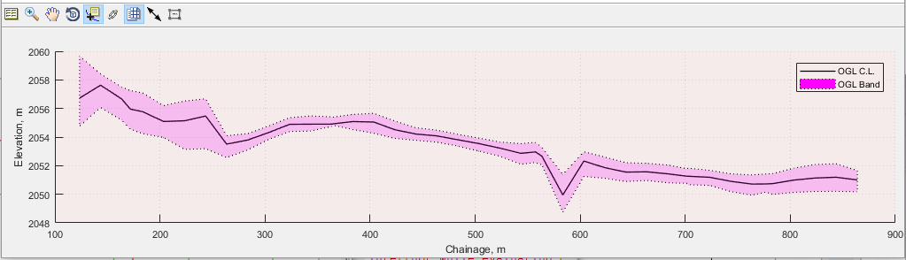
Note: If offset stations are provided, the profile will be plotted along with a band data indicating the variation of the ground level in the transverse direction.
When done, go to Sessions > Save to save the extracted profile data. This will save the data to the alignment route object itself. The object can then be used as a source object for further design or analysis work, as for example in canal reach design.
:bulb: Note: For Save to be successful, the alignment route object should already be in the current collection of iCAD workspace. If an object is listed in the left box in unguided mode, it is in the current collection. If not, use Workspace > Pick Collection or CTRL+K to add objects to the current collection.
Modify extracted data
You may want to modify an already extracted data often. For instance when the alignment route has changed its coordinates, or you want the data at a finer resolution. To modify or update profile data, simply repeat the process.
1. Invoke the module from CAD Tools > Extract Profiles. Provide the inputs as shown earlier.
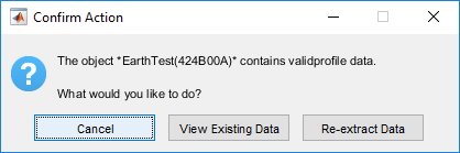
- The Confirm Action dialog will appear. Choose Re-extract Data. This will bring the Edit Variables dialog with the profile data specification variables. Input your new values, click apply and continue.
You will see the newly extracted profile. Save your work, before you exit.
Tip: You can use this process, to view/review an existing profile data on an alignment object. In the above Confirm Action dialog, choose View Existing Data.
2.5D Profile data generation
iCAD can also generate strip profile using a 2D profile data (along a center line) .This method helps when there is no cloud data source available, and only centerline profile data is available. Consider the center line profile data as shown in the figure below.
-
First, create a tentative layout object of comparable scale. (See Creating Local Axis chapter earlier in this section to learn how to create axes and associate objects to it.) This object will host the profile data you will generate.
-
Start CAD Tools > Extract Profile. Choose the center line profile as the cloud source, and the layout object as the Plan Layout object. Choose or set the desired offset locations for the strip profile generation.
 {br}
{br} -
Set extraction variablesto your needs, or accept the defaults. Choose Apply and continue.
-
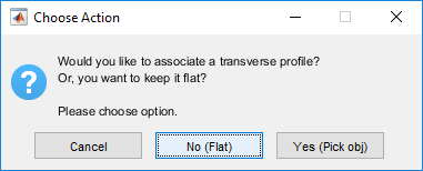
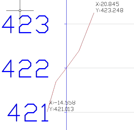
On the Choose Action dialog, you can choose to specify an object for transverse profile, or choose to make it flat. For illustration, a small profile is prepared on the vertical axis (shown in zoom) extending between -14.5 and 20.8, covering the offset dimensions specified above.
Note: Duing data generation, the transverse profile object at its STA=0.0 is snapped to the centerline elevation profile at each increment point. Hence, the variation of elevation is important rather than the elevation at which it is drawn.
Choose Yes (Pick Obj). AutoCAD will be in Select mode. Go to AutoCAD and pick the transvers profile object.
The profile is generated, as shown. You can save and use data
Batch processing profiles
iCAD version 1.9.8 includes a new feature, called Instantiation, to help in batch processing some tasks. Profile extraction is one of them.
Batch processing in profile data extraction is generation of profile data for more than one alignment route objects in one-go. This is most helpful for instance when preparing a system of canal layouts for design. Essentially, the preferences and data extraction settings will apply to all profile data. To use this method.
- Prepare all your layout objects, as you would normally for profile data extraction. This includes, referencing to a common axis. Then instance all the alignment objects using a host object. (See Using CAD Objects Extractor, Instantiation in this section).
-
Start CAD Tools >Extract Profile. Choose your cloud source, and offset settings as you would normally. Choose the instance object for Plan Layout variable. Continue to generate the profile for objects. A progress bar will show status.
Note: The profile data for each Alignment object is generated and saved automatically. There will be no preview or interim processing of the data. Use the steps discussed above to view/review the extracted data.
Data Visualization and Presentation
List data visualizaiton and presentaiton
List Data - from spreadsheet applications or CSV files, can be viewed in the iCAD environment with ease. Data sources can be AutoCAD objects hosting results of a pre-run iCAD module, e.g., ChannelRate_WSPRO hosting stage discharge relationships; or a data table from an MSExcel worksheet.
To use this functionality, start from CAD Tools > Plot/View Data. On the JET input dialog, select your data source. If data is in windows clipboard, use Shift+Click to input cb or clipboard. Otherwise click on the cell, and AutoCAD will be on select mode. Pick the object hosting the data.
Once in DataLiveiw, each data series can be viewed or processed separately. Tools are accessible by right clcking on the data points.
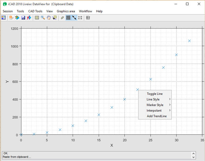
Toggle Line: Switches on/off the connecting line between data points
Line Style: Changes the line style of the connecting line (continuous, dashed, dash-dot, and dotted)
Marker Style: Changes the shape used to represent data points (Square, Circle, pentagram, or X mark.
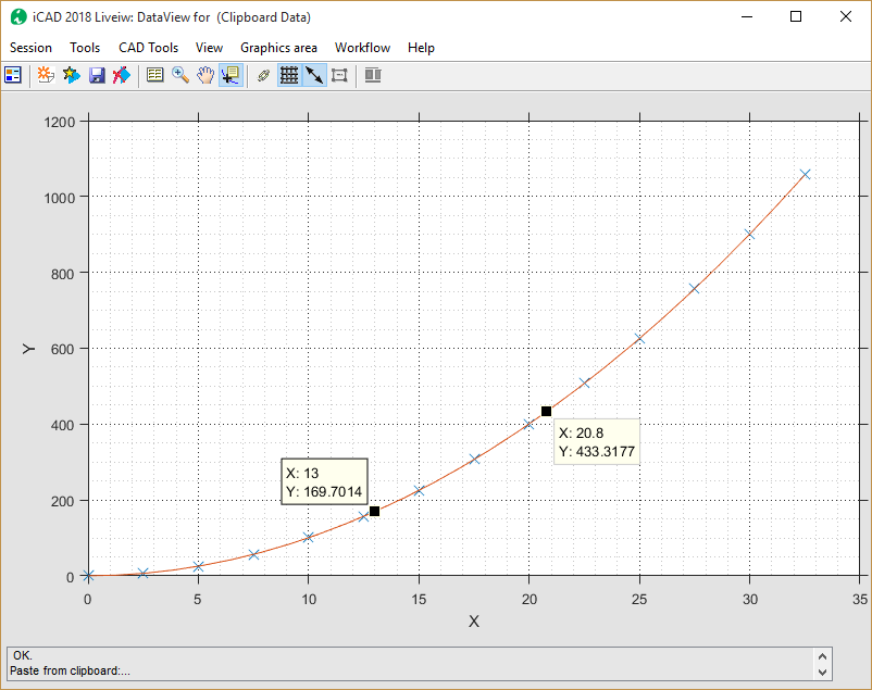
Interpolant: Specifies the interpolant function to use when creating the connecting line.
-
None: Use no interpolant (straight lines between data points)
-
Linear: Use linear interpolation with nearest neighborhood enabled
-
Cubic: Use cubic interpolation of neighborhood data points
-
Spline: Use spline interpolation of neighborhood data points
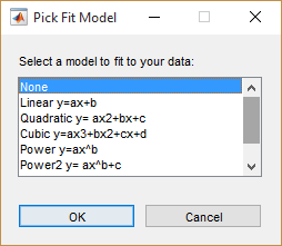
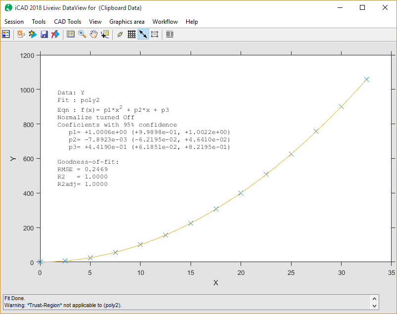
Trend line: This function fits a model to the data points in the series and display a statistics of goodness-of-fit.
The Interpolant feature is helpful when interpolating for intermediate values.
Trend line option displays the dialog to select a model from. A number of models are available to choose from. The statistics of the fit is displayed.
Note: The line style of the fit model, is similar to that of the data points.
Variables for Data visualization
| Variable Name | Description and remarks |
|---|---|
| Normalize Data | Allow or prevent data scaling and centering using mean and standard deviation of the data points |
| Exclude | A list of indices representing data points to exclude in computing model fit, such as outlier data points. This can contain up to 15 data indices. |
| Force Robust | On/Off: Enables or disables use of robust fitting method for the trend line (see note below) |
| Algorithm | Specify the algorithm to use in determining the best fit trend line: two options available.
|
| Axes Layout |
|
| Projection Data | A list abscissa values for which prediction is required using the fitted model. |
| Fit Extents | Dictates the range of abscisa values for which the model is computed.
|
| Flip Plot | This functionality allows easy flipping of data from the abscissa to the ordinate, and vice versa. See example beow. |
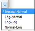 Scaling of the abscisa and
ordinate axes:
Scaling of the abscisa and
ordinate axes:Visual Presentation solutions for iCAD
iCAD main interface serves as a presentation and interaction medium for all its modules. The graphic contents in the interface can be enhanced for presentation purposes as follows:
-
Show Hide Elements
Users see the list of items plotted in the main interface from View > Graphics View Manager or
Ctrl+Mkeyboard short cut. Notice the displayed table at the bottom left corner.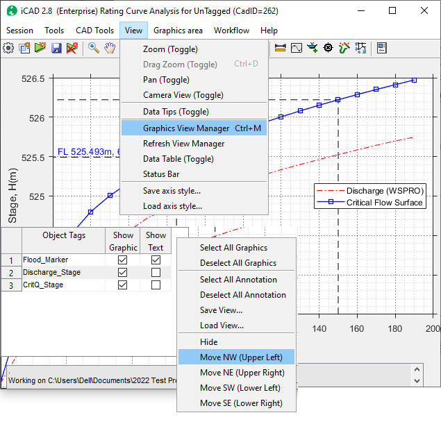
- Select/deselect the check boxes under Show Graphic column to show/hide the objects.
- select/deselect the check boxes under Show Text column to show/hide the texts pertaining to the object. Note that, this will not have any effect if the graphic of the object is not vissible.
- right-click on the table to display the options, and choose one of four alternative locations for the table (Upper Right, Upper Left, Lower Right, and Lower Left)
- to hide the table, right-click on it and choose Hide, or use the keyboard shortcut
Ctrl+M.
-
Data Cursor Tips
Users can label graohic elements using the Data Tips toolbar item or from the View > Data Tips (Toggle) menu item. Clicking on either will toggle the data cursor tip status for the graphic display area.
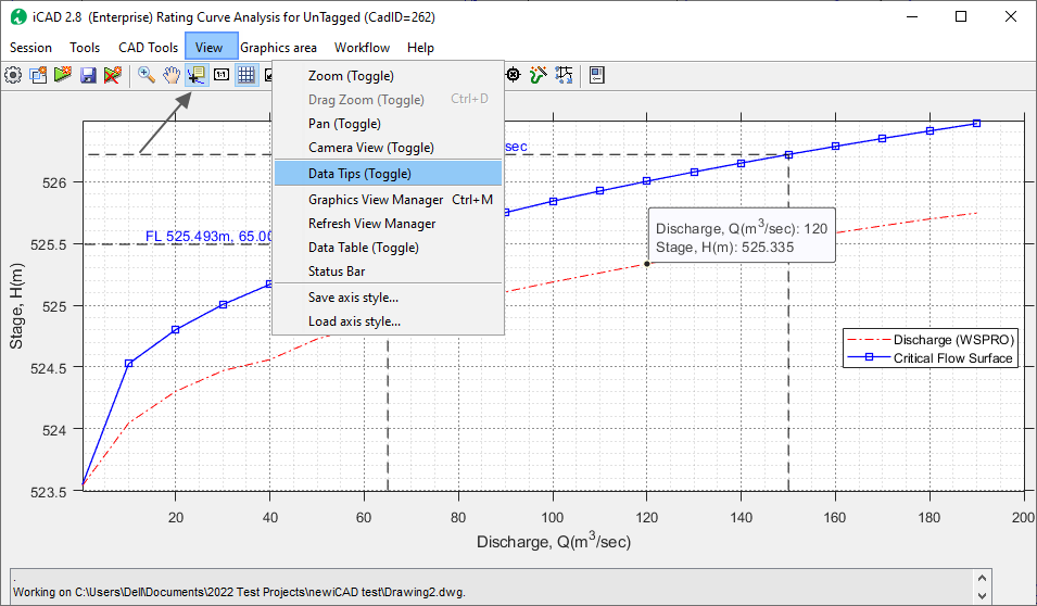
- To label graphic elements, toggle to ON, and hover on any graphic object. The cursor will change to a plus, indicating its ready to pick a point. Upon click, the data tip is inserted.
- To add more labels, hold any one of the shift/Ctrl/Alt keys while clicking on the object to label.
- to remove a data tip, right click on the data tip, and choose Delete Current Data Tip
- to remove all data tips, right click on any data tip, and choose *Delete All Data Tips
Note: By default, data tips can be positioned on data points only. To create data tips along lines, right click on any data tip, navigate to Selection Style and choose Mouse Position.
-
Copy Graphic area contetns
Users can copy the contents of the graphic window for various purposes. The following tools are available.
- Tools > Copy Graphics (To File) allows to save the current contents of the graphic area to a bitmap (.bmp) file.
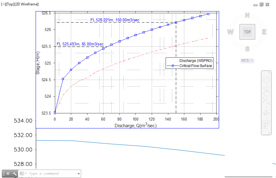
- Tools > Copy Graphics (To Clipboard) copies the contents of the current display to the windows clipboard. Use
Ctrl+Vkeyboard shortcut to paste the drawing to other applications such as word, excel or AutoCAD. The following figure shows such an image pasted to AutoCAD environemnt.
-
Generate Drawings to AutoCAD
Generally, all contents of the graphic area can be exported to AutoCAD and plotted at desired scaling.
- Use the Plot All to AutoCAD toolbar item to generate all the contents of the graphic area to AutoCAD. Notice the toolbar status message, indicating AutoCAD is in selection mode waiting for input
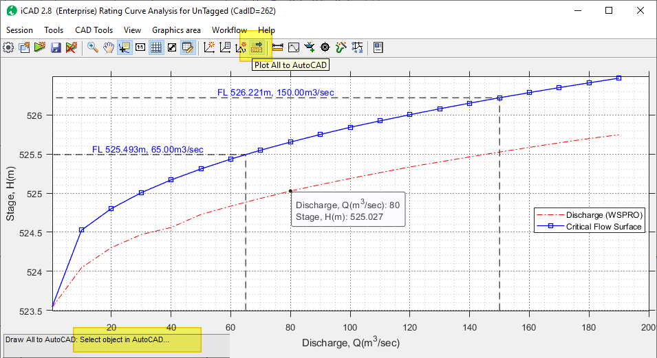
- In AutoCAD select a bounding box object.
- Pick a desired scaling, and create. If All scale value is used, the plot will be confined to the limits of this bounding box upon creation in AutoCAD. Otherwise, the objects are generated per given scaling with the origin set to the lower-left corner of the bounding box.
- Use the Plot All to AutoCAD toolbar item to generate all the contents of the graphic area to AutoCAD. Notice the toolbar status message, indicating AutoCAD is in selection mode waiting for input
An alternative method is available to plot individual objects to AutoCAD. This is available along with other workflow items for the active session, in Workflow > Select Draw to AitoCAD or Ctrl+P keyboard short cut.
Note: To use this method, a referenced object is required in AutoCAD.
Technical Notes: Fitting a Model or adding a trendline:
Fitting models to data points are based on certain assumptions, such as a normal distribution of errors in the observed responses. If the distribution of errors is asymmetric or prone to outliers, model assumptions are invalidated, and parameter estimates, confidence intervals, and other computed statistics become unreliable. The robust fitting method is less sensitive than ordinary least squares to large changes in small parts of the data.
Goodness-of-fit of the fitted model to a given data series, also called Coefficient of determination (R-squared), indicates the proportionate amount of variation in the response variable y explained by the independent variables X in the linear regression model. The larger the R-squared is, the more variability is explained by the regression model.
R-squared is the proportion of the total sum of squares explained by the model. R-squared, a property of the fitted model, is a structure with two fields:
Ordinary — Ordinary (unadjusted) R-squared
R^2^ = SSR/SST= 1-SSE/SST
Adjusted — R-squared adjusted for the number of coefficients:
R^2^= 1-(n-1)/(n-p)(SSE/SST)
- SSE is the sum of squared error, SSR is the sum of squared regression, SST is the sum of squared total, n is the number of observations, and p is the number of regression coefficients (including the intercept).
Because R-squared increases with added predictor variables in the regression model, the adjusted R-squared adjusts for the number of predictor variables in the model. This makes it more useful for comparing models with a different number of predictors.
RMSE – Root mean square error is a basic measure of how closely a model fits some data which measures the average mismatch between each data point and the model. High RMSE values can indicate problems. The smaller the RMSE, the closer our model follows the data; if a model goes through each data point exactly, then the RMSE is zero.
Notes (Flip Data):
A good application for the need of this variable can be demonstrated when fitting models to a stage-discharge relationship. Usually such data is available as shown in below table. One may copy such data to the windows clipboard (Ctrl+C), and visualize such data.
| (1) | (2) | (3) | (4) | (5) | (6) | (7) | (8) | (9) |
|---|---|---|---|---|---|---|---|---|
| Stage, H(m) | Depth, Y(m) | Discharge, Q(m^3/sec) | Flow Width, T(m) | Flow Area, A(m^2) | Velocity, V(x50 m/Sec) | Vel. Head, Vh(m) | Alpha | Conveyance, KD(m^3/sec) |
| 2052.224 | 0 | 0 | 0.000 | 0.000 | 0.000 | 0.000 | 0 | 0.0 |
| 2052.649 | 0.425 | 10 | 31.948 | 8.896 | 56.200 | 0.064 | 1 | 316.0 |
| 2052.802 | 0.578 | 20 | 35.932 | 14.138 | 70.700 | 0.102 | 1 | 632.2 |
| 2052.916 | 0.692 | 30 | 37.326 | 18.313 | 81.900 | 0.136 | 1 | 948.2 |
| 2053.014 | 0.79 | 40 | 38.530 | 22.050 | 90.700 | 0.167 | 1 | 1264.5 |
| 2053.101 | 0.877 | 50 | 39.437 | 25.443 | 98.250 | 0.197 | 1 | 1579.7 |
| 2053.18 | 0.956 | 60 | 39.973 | 28.551 | 105.050 | 0.225 | 1 | 1896.3 |
| 2053.253 | 1.029 | 70 | 40.473 | 31.485 | 111.150 | 0.252 | 1 | 2212.8 |
| 2053.321 | 1.097 | 80 | 40.944 | 34.284 | 116.650 | 0.277 | 1 | 2529.8 |
| 2053.386 | 1.162 | 90 | 41.386 | 36.942 | 121.800 | 0.302 | 1 | 2843.7 |
| 2053.448 | 1.224 | 100 | 41.813 | 39.537 | 126.450 | 0.326 | 1 | 3161.6 |
| 2053.507 | 1.283 | 110 | 42.217 | 42.019 | 130.850 | 0.349 | 1 | 3475.9 |
| 2053.565 | 1.341 | 120 | 42.611 | 44.456 | 134.950 | 0.371 | 1 | 3793.7 |
| 2053.62 | 1.396 | 130 | 42.989 | 46.825 | 138.800 | 0.393 | 1 | 4111.3 |
| 2053.673 | 1.449 | 140 | 43.355 | 49.125 | 142.450 | 0.414 | 1 | 4427.2 |
| 2053.725 | 1.501 | 150 | 43.705 | 51.354 | 146.000 | 0.435 | 1 | 4740.4 |
| 2053.775 | 1.551 | 160 | 44.050 | 53.561 | 149.350 | 0.455 | 1 | 5057.1 |
| 2053.821 | 1.597 | 170 | 44.630 | 55.609 | 152.850 | 0.476 | 1 | 5373.6 |
| 2053.866 | 1.642 | 180 | 45.986 | 57.645 | 156.100 | 0.498 | 1.002 | 5689.4 |
| 2053.91 | 1.686 | 190 | 47.315 | 59.700 | 159.100 | 0.519 | 1.005 | 6006.4 |
Notice:
-
The data must be selected without the column numbers at the top (1) to (9), which are added here for convenience of reference.
-
Velocity column is listed multiplied by 50x for ease of visibility

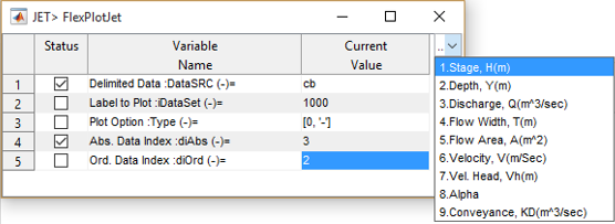
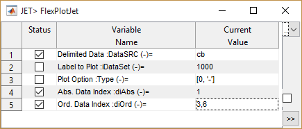
The standard way to visualize stage-discharge relationship is Discharge on abscissa and stage on the ordinate axes. But our data comes with Stage in the first column and discharge on the third column. It is possible to specify data indices in the JET dialog as follows to view stage-vs-discharge relationship.
The challenge comes to superpose a second series of data, say stage-vs-velocity. The two challenges are:
-
The abscissa index cell only takes the first indices even if you mention 3,6 only 3 (in this case representing Discharge column will be read.).
-
Data is plotted, using the abscissa value from the base column, and ordinate value from the value column. Requesting two sources for the abscissa value does not work.
The flip options solves this problem easily. Simply specify abscissa and ordinate column values as you would normally, i.e., 1 for abscissa and 3, 6 for ordinate.
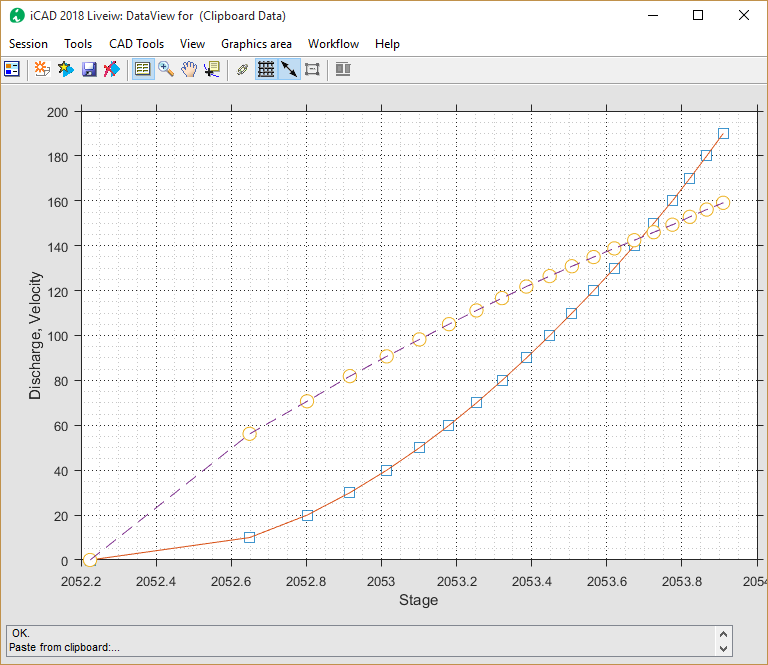
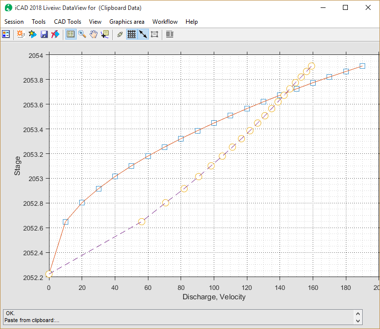
The resulting plots are shown below, with Flip set to noFlip and yesFlip respectively. As can be seen the second plot on the right is a more appropriate representation of the data.
Using CAD Objects Extractor
The CAD Object extractor module helps to explore and use AutoCAD objects and their properties in the iCAD workspace. The most common use of the module is to extract geometric properties, such as area, length or vertex coordinates and make this data available for subsequent processing.
Collecting and Managing Objects in to the Extractor
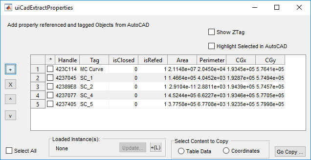
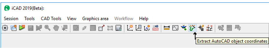
Start the interface from CAD Tools>Extract CAD Objects or from the toolbar menu Extract AutoCAD object Coordinates.
To add objects:
-
Use [+] button. AutoCAD will be in select mode.
-
Pick the object(s) you want, and right-click when done. The objects are read in to the interface and their property displayed.
Note: Only polyline objects can be collected in to the table.
To remove object(s):
-
Select the checkbox for the object you want to remove from the list
-
Use the [x] button.
Tip: You can check/uncheck the Select All checkbox at the bottom left, to select or deselect the whole collection.
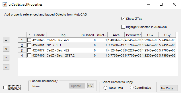
To manage display and highlighting, use below tools:
-
Show ZTag: Normally objects are listed using the Tag information provided in AutoCAD. Alternatively you can view the elevation of the objects by checking this box. The table would change as shown.
Note: You have to select objects after checking the box.
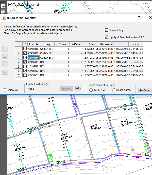
-
Highlight objects in AutoCAD: This interactive feature highlights the currently selected object(s) in the table in AutoCAD.
Exporting Data
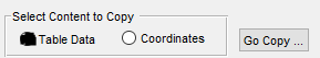
The following data can be obtained from the collected objects:
Export the table as is for use in a word or excel document.
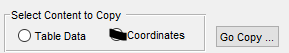
Check the Table Data radio (circle marker)
-
Click on Go Copy… button.
-
Go to you word or excel document and paste.
Extract and export coordinates of the selected objects:
-
Check the Coordinates radio button
-
Click Go Copy… button.
-
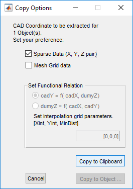
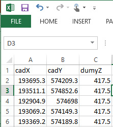
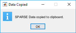
Choose Sparse Data (X,Y,Z pair) and click on Copy to clipboard.
-
Go to your word or excel document and paste.
Note: This tool allows to extract parametric plots for further processing. A useful application is in digitizing design charts. Request advanced features guide for details.
Instantiation
In version 1.9.8 and latter, a new feature is included in iCAD software called instantiation. This process allows representing different AutoCAD objects in one host object, called the instance object. This feature allows batch processing for many tasks including:
-
Reference objects
-
Import to workspace
-
Import to CAD extract
-
extract profile
-
Extract BoQ
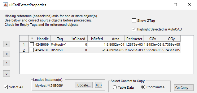
The CAD Extract interface allows to interactively manage instantiation of objects. To use it:
-
Clear contents and add an instance object. The instance object is imported along with the instanced objects. Here an object hosting one other object named Block50 is shown.
Note: The Loaded Instances panel is populated and the update button activated.
-
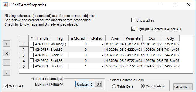
Add the other objects in AutoCAD that you want to append to the host or instance object (denoted with (+) suffix). You can do this using the [+] button as described above. For this example four farm blocks are added to the list.
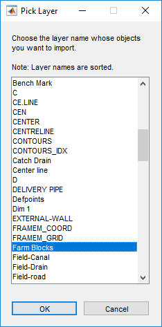
Alternatively, use the +[L] button at the bottom row to import objects contained in a Layer. In the Pick Layer dialog, select the layer containing your objects and click OK. This will import all objects on the selected layer to the CAD Extract table.
Tip: Manually remove any objects that you do not want in the group using [x] button.
-
Clcik on the Update button. This will signal that you want to instantiate all listed objects to the host object.
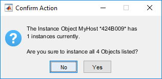
-
Click Yes on the Confirm Action dialog.
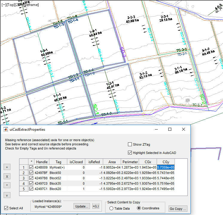
Check the contents of the host object after the update simply clear the contents using [x] button. Then add the host object using [+] button. The object now brings with it all 5 objects in to the table.
END.